Everything about Vlookup For Dummies
array _ lookup: It is defined whether you want an exact or an approximate suit. The possible worth holds true or FALSE. Truth value returns an approximate match, as well as the FALSE worth returns a specific match. The IFERROR feature returns a value one defines id a formula assesses to a mistake, otherwise, returns the formula.
IFERROR look for the list below mistakes: #N/ A, #VALUE!, #REF!, #DIV/ 0!, #NUM!, #NAME?, or #NULL! Note: If lookup _ value to be searched occurs more than once, then the VLOOKUP feature will certainly situate the first incident of lookup _ value. Below is the IFERROR Solution in Excel: The disagreements of IFERROR function are clarified listed below: worth: It is the value, recommendation, or formula to inspect for an error.
While utilizing the VLOOKUP feature in MS Excel, if the value looked for is not discovered in the provided data, it returns #N/ A mistake. Below is the IFERROR with VLOOKUP Solution in Excel: =IFERROR( VLOOKUP (lookup _ value, table _ selection, col _ index _ num, [range _ lookup], value _ if _ mistake) IFERROR with VLOOKUP in Excel is really easy and also easy to use.
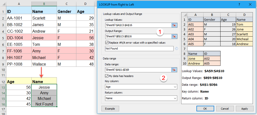
You can download this IFERROR with VLOOKUP Excel Design Template below-- IFERROR with VLOOKUP Excel Template Let us take an example of the standard pay of the workers of a company. In the above figure, we have a checklist of worker ID, Staff member Call and Employee basic pay. Now, we wish to search the workers 'basic pay relative to the Worker ID 5902. In this circumstance, VLOOKUP function will return #N/ An error. So it is far better to change the #N/ A mistake with a personalized worth that everybody can comprehend why the error is coming. So, we will certainly make use of IFERROR with VLOOKUP Function in Master the following means:=IFERROR (VLOOKUP (F 5, B 3:D 13, 3,0)," Data Not Discovered" )We will certainly observe that the mistake has actually been replaced with the personalized value "Information Not Found". We can use the function in the very same workbook or from different workbooks by the usage of 3D

cell referencing. Allow us take the instance on the very same worksheet to comprehend the usage of the function on the fragmented datasets in the same worksheet. In the above figure, we have two sets of information of basic pay of the workers. Now, we want to look the employees' standard pay relative to the Worker ID
Vlookup Fundamentals Explained
5902. We will make use of the following formula for searching data in table 1:=VLOOKUP (G 18, C 6: E 16, 3, 0)The result will certainly come as #N/ A. As the data looked for is unavailable in the table 1 information collection. The worker ID 5902 is available in Table 2 information established. Currently, we intend to contrast both of the information sets
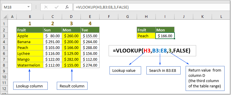
of table 1 and table 2 in a solitary cell and also get the result. It is better to replace the #N/ An error with a tailored value that everybody can comprehend why the error is coming. So, we will utilize IFERROR with VLOOKUP Function in Master the following method:=IFERROR(VLOOKUP(lookup _ worth, table _ range, col _ index _ num, [range _ lookup], IFERROR (VLOOKUP (lookup _ worth, table _ variety, col _ index _ num, [array _ lookup], value _ if _ mistake)) We have used the function in the example in the following way: =IFERROR(VLOOKUP(G 18, C 6: E 16, 3,0), IFERROR (VLOOKUP (G 18, J 6: L 16, 3, 0),"Information Not Discovered"))As the staff member ID 5902 is offered in the table 2 data set, the outcome will certainly show as 9310. Pros: Beneficial to catch and handle mistakes created by various other formulas or functions. IFERROR checks for the list below errors: #N/ A, #VALUE!, #REF!, #DIV/ 0!, #NUM!, #NAME?, or #NULL! Disadvantages: IFERROR replaces all sorts of mistakes with the tailored value. If any kind of other errors other than the #N/ An occur, still the tailored value specified will certainly be checked out in the result. If worth _ if _ mistake is offered as a vacant message(""), absolutely nothing is shown also when an error is found. If IFERROR is provided as a table range formula, it returns an array of results with one item per cell in the value field. This has been a guide to IFERROR with VLOOKUP in Excel. You can additionally govia our various other suggested short articles-- How to Use RANK Excel Function Function HLOOKUP Feature in Excel With Instances How To Use ISERROR Function in Excel. VLOOKUP is an incredibly beneficial formula in Excel. Regrettably -- for the SEM beginner-- it is also one of the most confusing when you are simply beginning. Because I 'm a loved one novice in paid search, the force of my job is production jobs. VLOOKUP is something that I make use of every single day. Naturally I requested aid, yet finding out VLOOKUP from somebody that currently recognized it as well as its ins and outs showed to be not so practical. I frantically wanted someone to just lay it out in the simplest, most stripped-down method feasible. So that's what I will do for you below: I'll walk you with the framework steps that I desire I had known. I don't even recognize everything it can do yet. )According to Excel's formula summary, VLOOKUP"tries to find a value in the leftmost column of a table, as well as after that returns a worth in the exact same row from a column you specify. "Super valuable, ideal? To stupid it down for you
, VLOOKUP lets you draw info concerning your picked cells into your existing sheet, from other sheets or workbooks where that value exists. CPC for each and every search phrase is. You have one more sheet that is a keyword report with all the data for every keyword phrase in the account-- this will certainly be called Keyword Sheet. You can stay clear of by hand filtering through all of those keyword phrases and needing to replicate and also paste the Avg. CPCs by utilizing VLOOKUP.
vlookup in excel openoffice excel vlookup duplicates excel vlookup left column